Interactive browser demo
From wrist IMU signals to activity records
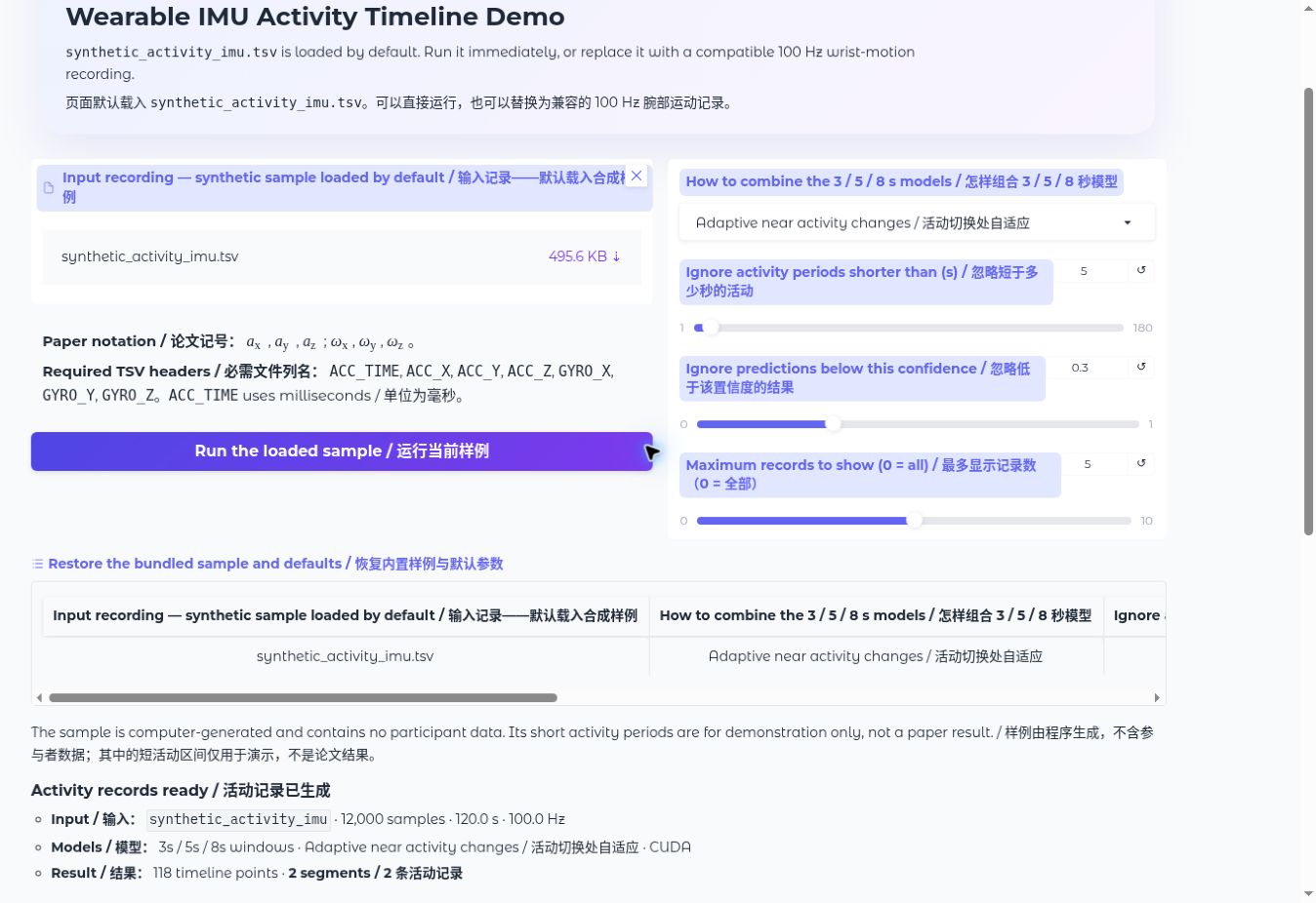
The bundled synthetic_activity_imu.tsv recording is loaded by default. Run it immediately, or replace it with a compatible 100 Hz wrist-IMU file.
 Actual bundled example
Run the bundled example
The fastest way to understand the interface is to run the deterministic synthetic_activity_imu.tsv example. It contains 12,000 samples, covers 120 seconds at 100 Hz, and contains no participant data. The live Space opens with this file already selected.
Select English in the language switch at the top of the Space. The complete interface—including controls, status messages, validation errors, result-table headers, and CSV export—then stays in English.
Open the Space
Open the live Demo and wait until the Gradio interface is ready.
Open live Demo ↗Confirm the preloaded sample
The file input already contains synthetic_activity_imu.tsv. Upload another file only if you want to test your own compatible recording.
Keep the defaults
Use local_boundary, minimum duration 5 s, confidence 0.30, and Top-K 5.
Run the current recording
Click Run current recording, then inspect the three result tabs.
Use Reset to synthetic sample at any time to restore the bundled file and all five defaults.
What happens after you click Run
The Space validates the preloaded file, loads the public checkpoints, runs the 3-, 5-, and 8-second models, fuses their posterior trajectories, applies the Temporal Record Layer, and returns plots, records, and a CSV in one request.
Reproducible example output
The figures below were exported from the current public checkpoints with the settings shown above. This run produced 118 timeline points and two activity records.
Demonstration, not validation
The sample is synthetic and is intended to show the complete input-to-output path. Its detected labels and boundaries are model outputs, not ground-truth accuracy evidence. Changing fusion, duration, confidence, or Top-K can change the records.
1. Raw signals
Open the first result tab to inspect the six channels before classification. The upper panel contains the acceleration channels \(a_x,a_y,a_z\); the lower panel contains the angular-velocity channels \(\omega_x,\omega_y,\omega_z\).
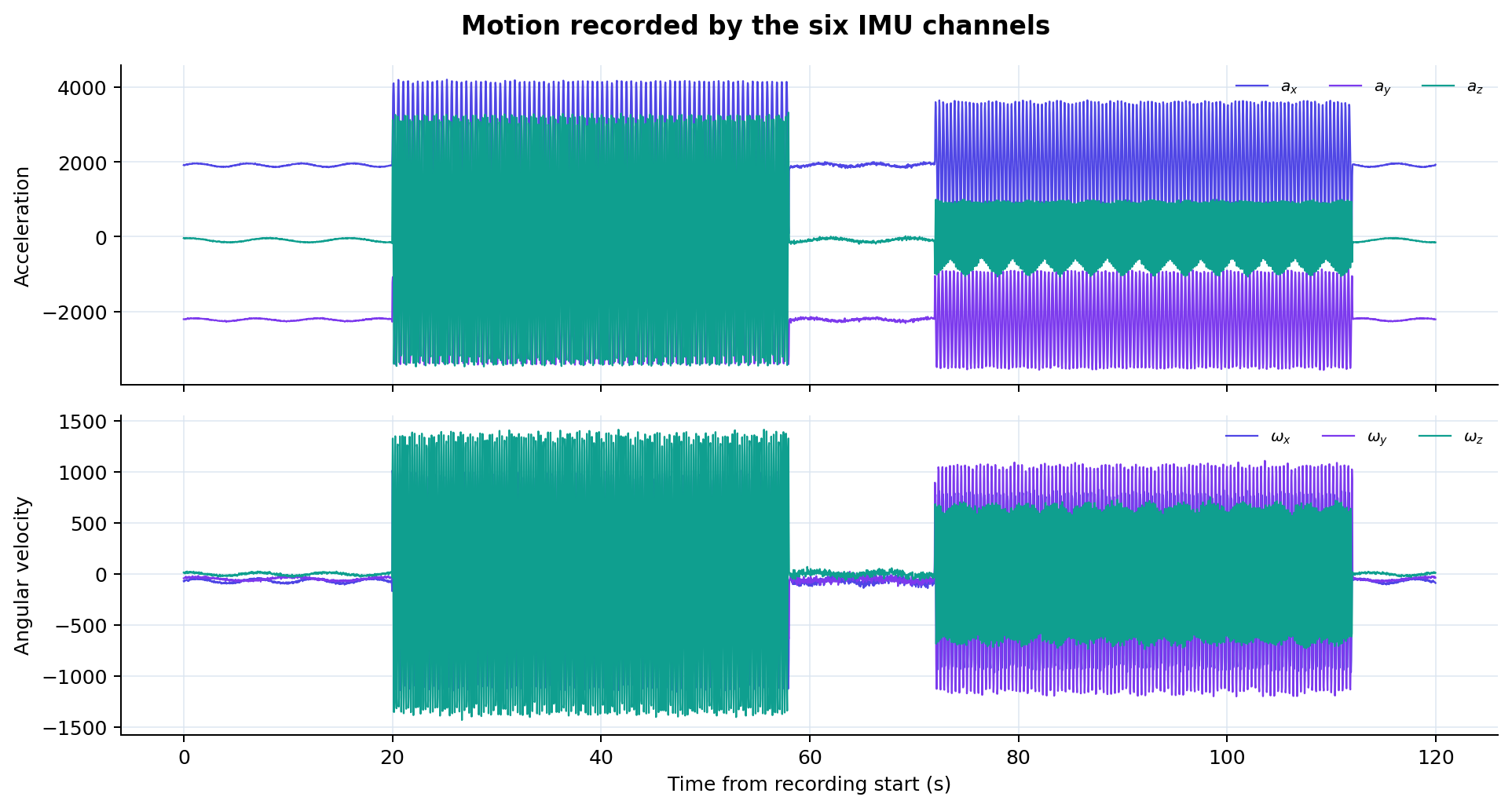
Quiet intervals appear near the beginning, between the two motion blocks, and at the end. Large periodic oscillations mark the two synthetic high-motion regions.
Use it to check missing channels, clipped values, unexpected offsets, sampling problems, and whether the uploaded recording contains visible motion.
2. Activity likelihood and timeline
The second tab shows two related outputs. The upper panel is the smoothed likelihood assigned to each class over time. The lower panel is the final decoded state after multi-scale fusion and temporal post-processing.
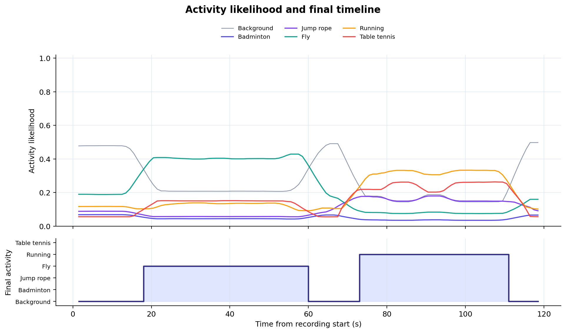
Background is strongest during quieter intervals. The first motion region raises the Fly likelihood, while Running becomes the strongest foreground likelihood in the second region.
The decoded path suppresses rapid label changes and returns a stable sequence: background, Fly, background, Running, then background.
3. Activity records
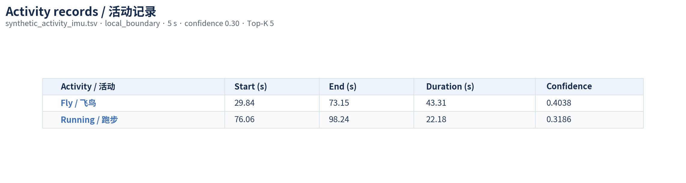
The third tab converts the decoded path into the output people can use: one row per activity period, with its class, start, end, duration, and confidence.
| Activity | Start (s) | End (s) | Duration (s) | Confidence |
|---|---|---|---|---|
| Fly | 29.84 | 73.15 | 43.31 | 0.4038 |
| Running | 76.06 | 98.24 | 22.18 | 0.3186 |
The record boundaries are not copied from the sample generator. They are produced by the model probabilities, Viterbi decoding, gap handling, boundary refinement, duration filtering, and confidence filtering.
What the controls change
| Control | Example setting | Effect |
|---|---|---|
| Model fusion | local_boundary |
Changes how the 3-, 5-, and 8-second posterior trajectories are combined, especially near possible transitions. |
| Minimum duration | 5 s |
Removes shorter decoded records. Raising it favors longer bouts; lowering it retains brief events. |
| Confidence threshold | 0.30 |
Removes weak records. Raising it may reduce false alarms but can also remove true low-confidence periods. |
| Top-K | 5 |
Limits the number of returned records after temporal processing; 0 disables this limit. |
The short settings above make the 120-second sample easy to inspect. They are Demo settings, not the fixed minute-scale settings used for the study results.
Use your own recording
- Prepare a UTF-8 tab-separated
.txtor.tsvfile. - Replace the preloaded synthetic file in the input control with your recording.
- Start with the Demo defaults, run once, and inspect Raw signals before interpreting the model output.
- Adjust one control at a time so its effect remains understandable.
Required columns:
The plots use paper notation: file columns ACC_X, ACC_Y, and ACC_Z are
shown as \(a_x,a_y,a_z\), while GYRO_X, GYRO_Y, and GYRO_Z are shown as
\(\omega_x,\omega_y,\omega_z\). The literal names above remain the required
TSV headers.
ACC_TIME must contain strictly increasing millisecond timestamps. The median interval must be 8–12 ms, corresponding to approximately 100 Hz. The public interface accepts 800–60,000 valid samples, or about 8 seconds to 10 minutes at 100 Hz. Extra columns are ignored.
Match the sensing protocol
A file can pass the format check and still be incompatible with the trained models. Sensor placement, axis orientation, units, device characteristics, and preprocessing should match the documented protocol. New devices, users, placements, and activities require new validation.
Privacy
Do not upload sensitive recordings
Do not send confidential or identifiable participant data to a public Space. Predictions are research outputs, not medical, safety, or coaching advice.
Run locally
Installation, verified model downloads, data boundaries, and local commands are maintained on the Reproduce page. The complete Gradio implementation is available in the repository's demo/ directory.