Method

The method converts a long wrist-IMU stream into a small set of activity records. It separates three questions: what the current motion resembles, which time scale is most reliable, and how window probabilities become stable start-to-end records.

\[ \begin{aligned} \mathbf{X} &\xrightarrow{\text{multi-scale posterior models}} \left\{ \mathbf{p}_{t}^{(3\,\mathrm{s})}, \mathbf{p}_{t}^{(5\,\mathrm{s})}, \mathbf{p}_{t}^{(8\,\mathrm{s})} \right\} \\ &\xrightarrow{\mathrm{LBSA}} \widetilde{\mathbf{p}}_{t} \xrightarrow{\mathrm{TRL}} \mathcal{R}. \end{aligned} \tag{1} \]

The complete signal \(\mathbf{X}\) produces three aligned posterior vectors; LBSA forms one fused trajectory and TRL converts it into the record set \(\mathcal{R}\).

IMU stream → multi-scale posteriors → LBSA → TRL → activity records.

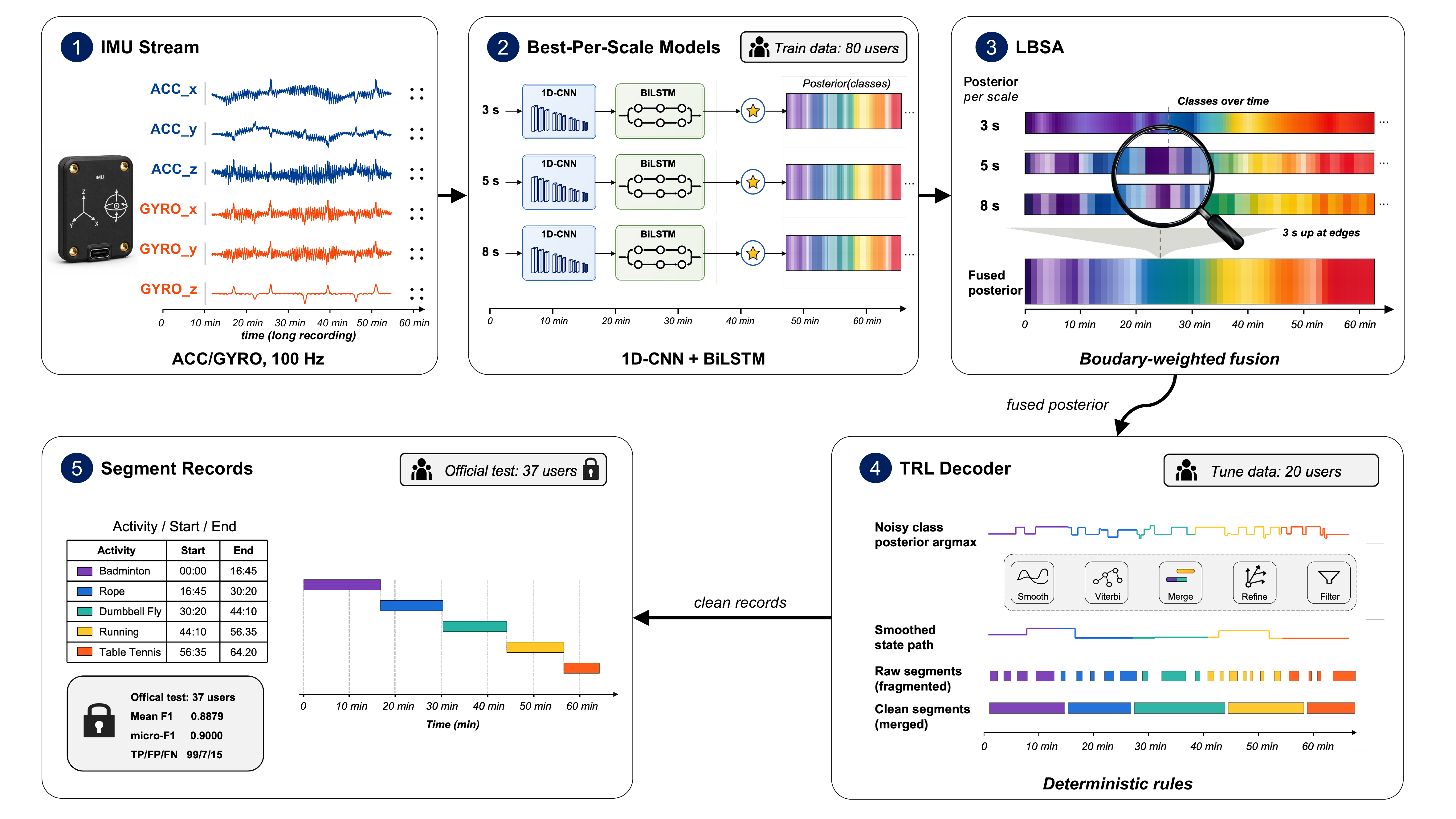
Task

The input is a 100 Hz stream whose six-channel sample vector is \(\mathbf{x}_t=[a_x(t),a_y(t),a_z(t),\omega_x(t),\omega_y(t),\omega_z(t)]^{\mathsf T}\). Here, \(a_x,a_y,a_z\) denote wrist acceleration and \(\omega_x,\omega_y,\omega_z\) denote wrist angular velocity along the three sensor axes.

The output is the variable-length record set \(\mathcal{R}=\{(c_i,t_i^{\mathrm{start}},t_i^{\mathrm{end}})\}_{i=1}^{N}\). This is temporal activity segmentation, not independent window classification. A useful system must recover the activity class, event count, duration, and boundaries of each workout segment.

Item	Definition
Sampling	100 Hz wrist acceleration and angular velocity
Window scales	3 s, 5 s, and 8 s
Step	1 s
Classes	background + five sports
Record match	same class, one-to-one, \(\operatorname{IoU}>0.5\)

Dataset

The study uses HLS-HAR, a long-session sports dataset collected with Huawei sports watches. It contains 137 recordings, about 46.8 million valid ACC/GYRO samples, and 259.6 hours of sensing.

Split	Recordings	Role
Training	80	fit models and select checkpoints during training
Development / calibration	20	tune and diagnose temporal policy
Independent external test	37	one final evaluation after all choices are frozen

The five foreground activities are badminton, rope skipping, dumbbell fly, running, and table tennis. The external set contains 114 labeled segments.

Posterior model

Each window is classified by a compact 1D-CNN + BiLSTM network with 1.41 million trainable parameters:

1. three temporal convolution branches use kernels 3, 7, and 15;
2. the branches capture short transients, rhythmic motion, and longer periodic cues;
3. a BiLSTM models the order of motion patterns across the window;
4. the fused head predicts background or one of five activities.

The same architecture is trained at all three scales. Short windows preserve transition detail; long windows provide steadier activity context. All scales advance by one second so their posterior trajectories can be aligned.

LBSA

Local-Boundary Scale Arbitration (LBSA) treats stable motion and transitions differently. The 5 s and 8 s posteriors are aligned to the 3 s grid. Away from transitions, longer windows receive more weight. Near a class change, the 3 s branch becomes dominant.

Region	3 s	5 s	8 s
Stable motion	0.20	0.35	0.45
Local boundary	0.50	0.27	0.23

At aligned time step \(t\), the fused posterior is a convex combination of the three scale-specific posteriors:

\[ \begin{aligned} \widetilde{\mathbf{p}}_{t} &= \sum_{s\in\mathcal{S}} \alpha_{t,s}\,\mathbf{p}_{t}^{(s)}, \\ \mathcal{S} &=\{3\,\mathrm{s},5\,\mathrm{s},8\,\mathrm{s}\}, \qquad \alpha_{t,s}\ge 0, \qquad \sum_{s\in\mathcal{S}}\alpha_{t,s}=1. \end{aligned} \tag{2} \]

The local boundary mask changes \(\alpha_{t,s}\): shorter evidence receives more weight near transitions, while longer context dominates stable motion.

The boundary mask comes only from posterior changes; it does not use segment labels. Temporal decoding is applied once, after the three scales are fused.

TRL

The Temporal Record Layer (TRL) converts the fused posterior trajectory into records through explicit, deterministic operations:

\[ \mathcal{R} = \operatorname{TRL}\!\left(\widetilde{\mathbf{p}}_{1:T}\right) = \left\{ \left(c_i,t_i^{\mathrm{start}},t_i^{\mathrm{end}}\right) \right\}_{i=1}^{N}. \tag{3} \]

Operation	Purpose	Paper setting
Moving average	suppress short probability dips	7 steps
Median filter	remove isolated spikes	kernel 5
Viterbi decoding	discourage rapid state switches	constrained transitions
Gap merging	join brief same-class interruptions	< 60 s
Boundary refinement	correct window-centering error	±15 s
Duration filter	remove short false records	≥ 180 s
Final pruning	limit weak or excess records	Top-K 3, confidence ≥ 0.45

These values encode minute-scale workout bouts; they are not universal HAR constants. New activity protocols require new calibration.

Measurement chain

Each stage controls a different record-level error:

Stage	Main uncertainty	Observable effect
Posterior model	ambiguous local motion	wrong or unstable class evidence
LBSA	scale-dependent boundary blur	shifted starts and ends
TRL	record construction	splits, merges, false alarms, and duration error

The final chain is evaluated with segment F1, matched IoU, boundary error, duration error, and false positives per hour. This keeps the reported evidence at the same level as the output people use: complete activity records.

Reproduction

Commands, file paths, and software interfaces are kept in Quickstart, Inference, and the API reference.